Introduction

Let us consider a problem, wherein we are interested in the missing values of the measurement of an experiment, that is being done. We want to take an ed- ucated guess about the missing value of the measurement. Let us illustrate this with an example that we encounter in our daily lives, of that being an athletic competition, in this case, the 1600 meters run. There are five measurements that are being done for each person. The four individual lap timings along with the total time taken to complete the race. Let us also suppose for some odd reason, there are missing values in terms of lap timings being measured in some cases and in some other cases, the total time taken to complete the race. We want to see if these missing values can be filled by some quantitative measure- ments. 

So for this data, if we proceed to create a matrix, with the athletes as rows and their lap timing for each lap as a column. As we can easily infer that the timings that we have are very close to each other, differing only by seconds or milliseconds. Now given the sampling of the data we would like to recover the matrix from the sampling, and in this case, the data is structured in such a way that the matrix is a low-rank one. This problem is akin to filling out the values of the matrix, and we try to complete the data based on the fact that the rank is low and can be solved by converting it to an optimization problem and solving it.

The above problem can be connected to the perimetry problem, if we take a small set of neighbouring points in the visual field the matrix formed by the threshold value of these points will be a low-rank matrix due to them having similar values this idea can be used to recover the whole matrix from a sampling of its entries.

A Note on Test Algorithms

The results of a test conducted on a test are affected by the following

• Device Characteristics: The results depend directly on how a specific de- vice works. A few factors include the absolute values of the incident in- tensities of light, the eye reliefs on the device. Device to device variation is captured by recording population normal on device hardware.

• Patient Reliability: The reliability of the patient determines the quality and accuracy of the test results obtained. Patient reliability is accounted for by performing catch trials (measurements that are designed to patient’s reliability and have no bearing on measurements)

• Test Method: The algorithm to begin, proceed and terminate the test has a very big effect on the final results that are used in the device.

The prototype V1.2 has an implementation of a measurement algorithm that is a variant of a Zippy Estimation of Sequential Thresholds(ZEST) method. This was implemented for the 24-2 pattern. The average test time on this algo- rithm was recorded to be about 15 minutes. Also, an error in the code resulted in incorrect measurement of patients with depressed fields. The existing algo- rithm is very slow and also only supports measurements at the moment. There is a need to improve the test algorithms to ensure good acceptance of the device. 

Speaking with interested customers in IIRSI, requirements for test algorithms were identified. Based on feedback from IIRSI, the algorithms need to be de- veloped to support the following
 

Test Patterns

Stratrgies 

White on White Perimetry.
 

Algorithms 

1. Screening algorithm to quickly identify patients with potential risk
2. Measurement algorithm to perform detailed measurements of the visual field to provide information for a comprehensive diagnosis.

Initially, the measurement algorithm is being fine-tuned as most screening tests are an adaptation of the measurement algorithm.
 

Algorithms 

In order to develop the best test algorithms, a state of the art search was conducted. Different features required for developing a robust test algorithm were identified and the best approach to integrate these features into our im- plementation was considered.
 

It must be noted that since the Mobile Perimeter is new hardware, that most of the parameters that relate to device characteristics/patient performance on the device are incorporated using careful informed assumptions. These parameters need to be updated once data from own devices are available.
 

The test algorithms that were studied were
 

1. The classic full threshold measurement used in Octopus Auto perimeter: this is a staircase method where the presented stimulus at a point is in- creased(decreased) by 4dB when the stimulus is seen(not seen). Once the stimulus value reaches a level where the presented stimulus is not seen(seen), the direction of the staircase changes and the stimulus value is decreased (increased) in 2dB steps. This process repeats with 1dB steps on the next reversal. Finally, the last seen stimulus is said to be the threshold value. [1]
    

2. The Humphrey full threshold measurement used by Humphrey: This is a variation of the classic threshold. Here the test proceeds in zones. It starts with 4 seed points in four quadrants. The results from these four points are used as seed points for neighbouring points once the tests are the four seed points are completed. More details can be found in the linked references by [2] and [6]
    

3. ZEST strategy with Bimodal Prior functions: A strategy based on the QUEST algorithm where a prior probability curve of expected threshold values at a location is used along with the information of the patient responses to determine the new probability curve for thresholds of the patient. More details can be found in the linked references by [7] , [8]
    

4. SITA standard based on published results: A famous well-accepted strat- egy that is a hybrid of staircase methods and ZEST strategies. References [9],[8].
    

5. Tendency oriented perimetry: New test strategy which is designed to be quick. The threshold at each point is modified 4 times where it is modified once based on response to the stimulus shown at the said location and three times based on the response to stimuli shown at neighbouring points.[10]
    

6. ZEST strategy with location-based weighted likelihood functions: A mod- ified ZEST procedure where the prior function of neighbouring points is also modified based on the response to a stimulus at a given point. [11]
    

7. Method incorporated in Prototype 1.2: Prototype 1.2 implemented a strat- egy based on the ZEST strategy with Bimodal prior functions (3 in this list).
    

8. New method: This will incorporate features from SITA standard (option 4) and ZEST strategy with location-based weighted likelihood functions (option 6).
    

Visual field test strategies involve many steps and different algorithms and com- panies have taken different approaches to each of these steps. The complete test can be divided into separate features in order to study and identify the approach best suited for the mobile perimeter.
 

The different features that are analyzed are
 

1. Test patterns: Test patterns define the points at which the visual field is tested. The test pattern to be used depends on the goal of the test and the make of the visual field analyzer.
    

2. Test pacing: Test pacing determines how quickly the test proceeds. Test pacing defines how long a stimulus is shown and the gap between the presentation of consecutive stimuli.
    



3. Reliability parameters: In every test, there is a need to estimate the re- liability of the test as it is possible for a patient to give wrong responses due to fatigue or being trigger happy. The reliability parameters that are tested are
    

1. False positives: If a patient responds “Seen” incorrectly, it is called a false positive. This can occur if a patient responds “Seen” for a stimulus that is not visible either due to low contrast or because it is not presented at all.
    

2. False negatives: If a patient does not respond to a stimulus that is expected to be seen, then it is considered as a false negative.
    

3. Fixation losses: If the patient moves his/her eyes during the test, then the resulting threshold measurements cannot be trusted because the visual field depends on the central fixation point. Fixation losses are measured by presenting supra-threshold stimuli at the expected blind spot of the patient.
    

4. Short term fluctuations: Inter-test variability is to be captured to evaluate patient attention over the course of the test.
    

4. Next point selection: At any point, there is a pseudo-random procedure with which the next point to be tested is determined by different test algorithms
    

5. Initial value at each point: The seed value/curve with which testing starts at given location
    

6. Post-processing after stimulus presentation: Based on the patient response to a given stimulus, the threshold value/curve at the said location is mod- ified. The new curve/value is used to determine the threshold value the next time this point is tested.
    

7. Determine end of testing at a given location: Once the post-processing of a stimulus presentation is done, a check is performed to determine if the test algorithm is done testing at that given location
    

8. Result estimation: If the test algorithm determines that a said location is to be released from testing, the final threshold curve/value is used to estimate the threshold result at the location
    

9. Fail back testing: Perimetry is known to result in widely varying results. In order to minimize the same, there are some fall back methods to minimize test variation.
    

This linked table details how each of the algorithms studied executes the said method, what has been implemented by us, and the plan for the algorithm that is being implemented.
 

UNITS 

The decibel range depends on perimeter type and typically ranges from 0 dB to approximately 32 dB in the fovea. A sensitivity threshold of 0 dB means that a patient is not able to see the most intense perimetric stimulus that the device can display, whereas values close to 32 dB represent a normal foveal vision for a 20-year-old person. The sensitivity to light in decibels is defined using the formula below
 

where dB is the sensitivity threshold, L max is the maximum luminance the perimeter can display, and L is the luminance of the stimulus at the threshold (both expressed in apostilbs). The logarithmic scale is used to address the large range of luminance values and to relate this range more linearly to visual function. To address the inverse relationship between luminance and sensitivity to light, the inverse of luminance (1/L) is used in the formula; and to make sure that near-complete visual field loss equals 0 dB, which is intuitive, the maximum stimulus luminance L max is added to the equation. 0 dB refers to the maximum intensity that the perimeter can produce
 

Test Algorithms 

Octopus Full Threshold 

Overview-The octopus Full Threshold strategy is a standard strategy used for perimetry tests. Initially, 4 points at 12.7 degrees from the central fixation point are tested. The test starts from an initial value which we take from the data at hand. Initially, the points are changed in intervals of +4 if seen, if the stimulus is not seen then the intensities are changed in the opposite direction but this time in intervals of 2 till the stimulus is seen , then again it is changed in intervals of 1 but in reversed direction. The last seen value is the threshold value. After this, the points neighbouring these points are tested, with the initial value being the result of the neighbouring test point.
 

1. Test pattern: Octopus specific
    

2. Test pacing: Fixed.
     100 ms stim. Duration
     1800 ms btw stim.
    

3. Reliability Parameters: -
    

   1. False Positives: Simulate a stimulus while not presenting.
       

   2. False Negatives: Present a supra-threshold value at a point that has already been executed.
       

   3. Fixation Losses: Active fixation monitoring
       

   4. Short term fluctuations: Not known
       

4. Next Point Selection: Zone wise. Initially, 4 points at 12.7 degrees from the central fixation point are tested. After this, the points neighbouring these points are tested. Once all the points in the second set are done, the third group consisting of neighbours of the previous point are tested and so on
    

5. Initial value/curve at each point: Only seed values are used for the first four points. These are based on age-based normative curves stored on the device.
     Remaining points are initialized using results from the neighbouring points.
    

6. On Seen/Unseen: On Seen/Unseen
    

7. Determination of end of testing: If at a given point there have been two separate reversals, then the testing at the point is said to finish. The entire test is supposed to have finished when all points go through two reversals
    

   1. If Yes, estimate result: The result at a point is the last seen stimulus
       

   2. If no, estimate the next level that is shown: The next level is equal to the value estimated post seen/unseen
       

8. Fail-safe methods: If the result value is more than 4dB different from the initial value, the test re-run at the point starting at the result value.
    

9. Post-processing: None
    

Humphrey Full Threshold 

OVERVIEW: The Full Threshold strategy is currently regarded as a standard technique in static threshold perimetry and is used in most glaucoma-related clinical trials. In this test strategy, a suprathreshold stimulus is presented at each location based on the threshold values from prior points. Intensity is decreased at fixed increments until the stimulus is no longer seen, and then increased at fixed increments until it is seen again. The threshold value is taken to be equal to the intensity of the last stimulus seen at that location.
 

WORKING: Initially, 4 points at 12.7 degrees from the central fixation point are tested. Initially, the points are changed in intervals of 4, if a stimulus is not seen then the intensities are changed in the opposite direction but this time in intervals of 2 till the stimulus is seen, then again it is changed in intervals of 1 but in reversed direction. The last seen value is the threshold value. After this, the points neighbouring these points are tested, and the initial value being the result of the neighbouring test point.
 

1. Test pattern: Humphrey specific (24-2,30-2,10-2,macula)
    

2. Test pacing: Fixed
     200 ms stim. Duration
     1800 ms btw stim.
    

3. Reliability Parameters: -
    

   1. False Positives: Simulate a stimulus while not presenting.
       

   2. False Negatives: Present a supra-threshold value at a point that has already been executed.
       

   3. Fixation Losses: Test at blind spot location using catch trials
       

   4. Short term fluctuations: 10 pre-determined points are tested twice and the difference is considered for the STF
       

4. Next Point Selection: Zone wise. Initially, 4 points at 12.7 degrees from the central fixation point are tested. After this, the points neighbouring these points are tested. Once all the points in the second set are done, the third group consisting of neighbours of the previous point are tested and so on
    

5. Initial value/curve at each point: Only seed values are used for the first four points. These are based on age-based normative curves stored on the device.
     Remaining points are initialized using results from the neighbouring points.
    

6. On Seen/Unseen: Update reversal number if unseen changed to seen or vice-versa.
     If seen:
     Add 4 or 2 or 1 decibels to the presented value based on presented value.
     If unseen :
    Subtract 4,2,1, based on reversal value

7. Determination of end of testing: If at a given point there have been two separate reversals, then the testing at the point is said to finish. The entire test is supposed to have finished when all points go through two reversals
    

   1. If Yes, estimate result: The result at a point is the last seen stimulus
       

   2. If no, estimate the next level that is shown: The next level is equal to the value estimated post seen/unseen
       

8. Fail-safe methods: If the result value is more than 4dB different from the initial value, the test re-run at the point starting at the result value.
    

9. Post-processing: None
    

ZEST using Bimodal PDFs 

Overview - The ZEST algorithm is widely used for testing in hospitals. Points are selected pseudo-randomly to make sure that the patients are not able to pre- dict the next pattern. For each stimulus location, an initial probability density function (pdf) is defined that states for each possible threshold, the probability that any patient will have that threshold. The pdf is a weighted combination of normal and abnormal thresholds. The normal pdf gives a probability for each possible patient threshold, assuming that the location is “normal”, whereas the abnormal pdf gives probabilities assuming the location is “abnormal”. abnor- mal pdfs, threshold estimates were pooled across all locations. For each test location, the abnormal and normal pdfs are combined in a ratio of 1:4. The ZEST procedure presents the first stimulus at an intensity equal to the mean of the initial pdf and then uses the subject’s response (seen or not seen) to modify the pdf. To generate the new pdf, the old pdf is multiplied by a likelihood func- tion (similar to a frequency-of- seeing curve), which represents the likelihood that a subject will see a particular stimulus. The process is repeated until a termination criterion is met(in this case, standard deviation of pdf \< 1.5 dB). The output threshold is the mean of the final pdf
 

1. Test pattern: Not Applicable
    

2. Test pacing: Not Applicable
    

3. Reliability Parameters: -
    

   1. False Positives: Simulate a stimulus while not presenting.
       

   2. False Negatives: Present a supra-threshold value at a point that has already been executed.
       

   3. Fixation Losses: Not Applicable
       

   4. Short term fluctuations: Not Applicable
       

4. Next Point Selection: Not Known
    

5. Initial value/curve at each point: Based on normal and abnormal databases, an abnormal and normal pdf is created. Procedure to create the pdfs is the following
    

   1. At each location, 95 percentile value
       

   2. Threshold values at all locations are pooled for all normal results and normal pdf is made
       

   3. Using < 95% value, abnormal values are captured and the threshold values at all locations are pooled to make the abnormal pdf.
       

   4. The mode of the normal pdf is shifted to the expected threshold value at each location and combined with abnormal pdf in a 4:1 ration
       

6. On Seen/Unseen: if seen, use the seen likelihood function which is 50% at the presented stimulus and multiply the prior curve. If not seen, do the same thing with the not seen likelihood function
    

7. Determination of end of testing: The standard deviation of the post function is calculated. If the SD is less than 1dB, it is said that the testing at the point is completed. The entire test is said to be done when all points are terminated.
    

   1. If Yes, estimate result: The mean of the final posterior curve is the threshold value
       

   2. If no, estimate the next level that is shown: the mean of the posterior curve
       

8. Fail-safe methods: None
    

9. Post-processing: None
    

SITA Standard 

OVERVIEW: It is a new family of test algorithms for computerized static thresh- old perimetry which significantly reduces test time without any reduction of data quality. The traditional perimetry tests used staircase method to find the threshold value at each point,which was time-consuming. The current project was to develop new algorithms for threshold determination, having considerably shorter test times and at least the same accuracy as current standard threshold tests by using maximum likelihood methods.
 

WORKING: The test procedure starts by measuring threshold values at four pri- mary points, one in each quadrant of the field at 12.7’ from the point of fixation. Stimulus intensities are altered in conventional up-and-down staircases. As the test goes on, last seen stimulus intensities in neighbouring points are used to cal- culate starting values in new points not previously opened for testing. Stimulus exposures at different test point locations are presented in pseudo-random order to prevent patients from predicting locations of coming stimulus presentations. Stimulus intensities are altered in staircase procedures at all test point locations. All responses, both negative and positive, are added to the model. The poste- rior probability functions are recalculated after each stimulus exposure at each test point, and also after stimulus exposures at adjacent points. Furthermore, all probability functions at all test points are recalculated periodically. These updated probability functions result in new MAP estimates of threshold values, in both the normal and the defective model. The influence of the prior model gradually decreases as more test data are added to the models. During the test, measurement error estimates are compared to a predetermined limit, called the error related factor(ERF), $$ ERF = a + b_1 × \sqrt{variance} − b_2 × threshold \,\, value$$ As soon as the measurement error at a given point is smaller than the ERF, the threshold value is considered to have been estimated to sufficient accuracy and testing is terminated. Different levels of accuracy can be obtained by varying the ERF value.
 

1. Test pattern: Humphrey Specific
    

2. Test pacing: The test usually takes place with a duration of 100ms for each stimulation and a delay of 1000-1400ms is given between each stim- ulation
    

3. Reliability Parameters: -
    

   1. False Positives: Use patient-specific response time windows to de- termine false positives
       

   2. False Negatives: Present a supra-threshold value at a point that has already been executed.
       

   3. Fixation Losses: Passive gaze monitoring. Check for fixation using camera at random
       

   4. Short term fluctuations: 10 pre-determined points are tested twice and the difference is considered for the STF
       

4. Next Point Selection: The initial point selection is done zone wise. Initially, 4 points at 12.7 degrees from the central fixation point are tested. After this, the points neighbouring these points are tested. Once all the points in the second set are done, the third group consisting of neighbours of the previous point are tested and so on.
   As the test goes on, last seen stimulus intensities in neighbouring points are used to calculate starting values in new points not previously opened for testing. Stimulus exposures at different test point locations are presented in pseudo-random order to prevent patients from predicting locations of coming stimulus presentations
    

5. Initial value/curve at each point: SITA standard has two components to initial values and initial curves.
    

   1. Initial values at 4 seed locations are determined by age-based nor- mal values
       

   2. The remaining points are determined by the result from the 4 seed values
       

   SITA standard also uses prior/initial curves. There are two of them
   

   Likelihood of normals and abnormals at each point compiled from pre- vious information
    

6. On Seen/Unseen: In SITA two things are done.
    

   Based on the number of reversals and whether the stimulus was seen/unseen, and a value of 4 or 2 db is added/subtracted to the present intensity value.
   

   In addition, the likelihood function based on the stimulus value presented is multiplied with both the prior curves (the abnormal prior function and the normal prior function)
    

7. Determination of end of testing: The testing at a point is said to end when there are two reversals in the change in intensity at the point
   or
   An error related function(ERF), $$ERF =a+b× \sqrt{variance}−b_2 × threshold \,\, value$$ that measures the dispersion on the two post functions is below a certain predefined value and there is at least one reversal
     The test ends when all points satisfy the condition.

   1. If Yes, estimate result: The higher mode of the two posterior curves is considered as the answer
       

   2. If no, estimate the next level that is shown: The value cal- culated using the staircase strategy post seen/unseen is used as the next presented threshold
       

8. Fail-safe methods: If the resulting threshold value is more than 12dB different from the initial value at that point, the test is re-run at the point starting from the result value.
    

9. Post-processing: All the posterior curves are redone using updated FOS curves
    

Tendency Oriented perimetry 

OVERVIEW: Tendency-oriented perimetry (TOP) is a new strategy designed to estimate the sensitivity of the visual field quickly, by using linear interpolation between test locations. The TOP algorithm uses a subject’s response at a given point, not only to estimate the sensitivity at that point, but also to modify the sensitivity estimate of surrounding points within the visual field.
 

WORKING: The procedure commences by assuming that the initial sensitivity estimate for each location is half the age-expected. The threshold at each point is modified 4 times where it is modified once based on response to the stimulus shown at the said location and three times based on the response to stimuli shown at neighbouring points. Stimuli from the first submatrix are presented, and the responses recorded; a “seen” response is recorded as 4/16 of the age- expected sensitivity at the location, and an “unseen” response is recorded as -4/16 of the age-expected sensitivity. Threshold estimates are then adjusted by the average response value, based on a 3x3 window centered on the point in question Testing then continues for points from the second submatrix, with responses recorded as 3/16 of the age-expected sensitivity. Threshold estimates then are adjusted, based only on the average responses from the second subma- trix, again using a 3x3 window. Responses from the third and fourth submatrices are similarly recorded as 2/16 and 1/16 of the age-expected sensitivity.
 

1. Test pattern: Specific to TOP. Uniformly distributed grid required for TOP
    

2. Test pacing: The test usually takes place with a duration of 100ms for each stimulation and a delay of 1800ms is given between each stimulation
    

3. Reliability Parameters: -
    

   1. False Positives: Simulate a stimulus while not presenting.
       

   2. False Negatives: Present a supra-threshold value at a point that has already been executed.
       

   3. Fixation Losses: Active fixation monitoring
       

   4. Short term fluctuations: Not Known
       

4. Next Point Selection: TOP operates within a uniform grid that is uniformly spread. All the points of each zone are tested at any point in time. Once all the points are tested, the test moves on to the next zone.
    

5. Initial value/curve at each point: In the TOP procedure, the visual field is divided into four overlapping submatrices. The procedure com- mences by assuming that the initial sensitivity estimate for each location is half the age-expected sensitivity value
    

6. On Seen/Unseen:Stimuli from the first submatrix are presented, and the responses recorded ; a “seen” response is recorded as \(+ 4 \over 16\) of the age- expected sensitivity at the location, and an “unseen” response is recorded as \(- 4 \over 16\) of the age-expected sensitivity. Threshold estimates are then adjusted by the average response value, based on a 3x3 window centered on the point in question.
   Testing then continues for points from the second submatrix, with responses recorded as \(\pm 3 \over 16\) of the age-expected sensitivity. Threshold estimates then are adjusted, based only on the average responses from the second submatrix, again using a 3x3 window. Responses from the third and fourth submatrices are similarly recorded as \(\pm 2 \over 16\) and \(\pm 1 \over 16\) age-expected sensitivity, respectively, and sensitivity estimates adjusted as outlined previously.  

7. Determination of end of testing: Stimulus presented at a point only once. Test ends when all points are tested
    

   1. If Yes, estimate result: Result is estimated based on the seen and unseen answers at the end of each stage of the test. The final threshold answer is the threshold estimated after stage 4, that is 4 sensitivity adjustment to a particular submatrix
       

   2. If no, estimate the next level that is shown: The result is a summation of factors based on the response at a given point and the responses at the neighbouring points
       

8. Fail-safe methods: None
    

9. SPost-processing: None
    

10. Result:The results of some simulations have showed that the TOP strat- egy has poor spatial resolution characteristics. Sensitivity estimates or small defects showed a characteristic bi stratification with the depth of the defect typically being underestimated. Sensitivities were estimated with greater fidelity as defect size increased
    The TOP strategy can reliably detect large contiguous scotomas such as those present in glaucoma. However, it smoothes the edges of the scotomas and is less sensitive to small, localized defects compared to a systematic sampling procedure such as the dynamic strategy
     

Spatially weighted ZEST 

OVERVIEW: The Zippy Estimation of Sequential Thresholds (ZEST) is a Bayesian forecasting procedure similar to SITA that has been implemented on the new Humphrey Matrix which uses frequency doubling technique. ZEST has been reported to demonstrate sensitivity, specificity, and reproducibility that is com- parable to other threshold estimation procedures while reducing test time by approximately 50 percent. The FDT version of ZEST appears to have some advantages over the SITA procedure as it is computationally and procedurally simpler than SITA.
 

WORKING: In case of zest algorithm before testing begins, each location in the visual field is assigned a probability mass function (PMF). The PMF defines the probability that each possible visual sensitivity value (5to40dB) is the true visual sensitivity of the observer. Note that, although negative intensity values cannot be physically tested, they are included in the domain to prevent a floor effect on visual sensitivity estimation. Negative dB values cannot be tested be- cause luminance values increase with decreasing dB values, and 0 dB represents the maximum intensity that the visual field machine can display. A bimodal PMF was created using a weighted combination of normal and abnormal visual sensitivity population data (4:1, respectively) The resultant curve has two peaks: one peak representing healthy visual sensitivities and another smaller peak rep- resenting dysfunctional sensitivities. During the test, stimuli are presented with an intensity equal to the mean of a location’s PMF. After each presentation, a new PMF is generated for the tested location by multiplying the current PMF by a likelihood function. The likelihood function represents the probability that the observer will see the stimulus and is defined by a cumulative Gaussian cen- tered on the test presentation intensity with a standard deviation of 1 dB. The test terminates when the standard deviation of the PMF at each location is 1.5 dB. The final estimate of visual sensitivity for each location is the mean of the final PMF for that location.
 

1. Test pattern: Not Applicable
    

2. Test pacing: Not Applicable
    

3. Reliability Parameters: -
    

   1. False Positives: Simulate a stimulus while not presenting.
       

   2. False Negatives: Present a supra-threshold value at a point that has already been executed.
       

   3. Fixation Losses: Not Applicable
       

   4. Short term fluctuations: 10 pre-determined points are tested twice and the difference is considered for the STF
       

4. Next Point Selection: Two major zones. 4 points at 12.7 degrees from the central fixation point are tested. Post that remaining points are chosen based on the spread of the prior threshold curves associated with them. In case of ties, the points are chosen at random.
    

5. Initial value/curve at each point: All points are initialized with a prior function using a peak at 0 decibels and a peak at 30 decibels.
    

6. On Seen/Unseen: If seen, then the prior curves as well as certain neigh- bouring points curves are multiplied with a weighted likelihood functions
    

7. Determination of end of testing: The standard deviation of the post function is calculated. If the SD is less than 1dB, it is said that the testing at the point is completed. The entire test is said to be done when all points are terminated.
    

   1. If Yes, estimate result: The mean of the final posterior curve is the threshold value
       

   2. If no, estimate the next level that is shown: the mean of the posterior curve
       

8. Fail-safe methods: None
    

9. Post-processing: None
    

Mobile Perimetry Prototype 1.2 

1. Test pattern: Similar to Humphrey (only 24-2)
    

2. Test pacing: Fixed.
   100 ms stim. Duration
   1950 ms btw stim.  

3. Reliability Parameters: -
    

   1. False Positives: Simulate a stimulus while not presenting.
       

   2. False Negatives: Present a supra-threshold value at a point that has already been executed.
       

   3. Fixation Losses: Test at blind spot location using catch trials
       

   4. hort term fluctuations: Not Implemented
       

4. Next Point Selection: Zone wise. Initially, 4 points at 12.7 degrees from the central fixation point are tested. After this, the points neighbouring these points are tested. Once all the points in the second set are done, the third group consisting of neighbours of the previous point are tested and so on
    

5. Initial value/curve at each point: The Four seed points were initiated with a bimodal pdf with a mode of the normal pdf at 22 dB.
   Post that the different zones were estimated using results from neighbouring points.  

6. On Seen/Unseen:
   if seen, use the seen likelihood function which is 50% at the presented stimulus and multiply the prior curve.
   If not seen, do the same thing with the not seen likelihood function  

7. Determination of end of testing: The standard deviation of the post function is calculated. If the SD is less than 1dB, it is said that the testing at the point is completed. The entire test is said to be done when all points are terminated.
    

   1. If Yes, estimate result: The mean of the final posterior curve is the threshold value
       

   2. If no, estimate the next level that is shown: The mean of the final posterior curve is the threshold value
       

8. SFail-safe methods: Non
    

9. Post-processing: None
    

Mobile Perimetry Final 

1. Test pattern: Similar to Humphrey (30-2,24-2,10-2,Macula)
    

2. Test pacing: Variable. (based on patient response)
   150 ms stimulation Duration
   1000-1500 ms btw stim.  

3. Reliability Parameters: -
    

   1. False Positives: Simulate a stimulus while not presenting.
       

   2. False Negatives: Present a supra-threshold value at a point that has already been executed.
       

   3. Fixation Losses: Active fixation monitoring
       

   4. Short term fluctuations: Not planned
       

4. Next Point Selection: Zone wise. Initially, 4 points at 12.7 degrees from the central fixation point are tested. After this, the points neighbouring these points are tested. Once all the points in the second set are done, the third group consisting of neighbours of the previous point are tested and so on
    

5. Initial value/curve at each point: The new algorithms includes values considering the new dimensions as well as prior distribution curves.
    

   1. Normals at each point are considered based on published data from Humphrey team. The log scales differences will be accounted for. It is going to be assumed that the slopes of decrease in sensitivities due to age remain constant.
       

   2. Normal curves are generated at each location using the information available (mean at 50 years age and standard deviation at 50 years age). Skewness and kurtosis of this deviation is estimated using the single per- centile distribution available in the published data.
       

   3. Abnormal curves are being generated using humphrey reports and compiling data of all the values that are below < 5% in total deviation plots
       

6. On Seen/Unseen: In SITA two things are done.
   Based on reversal number and seen/unseen state 4 or 2 db is added/subtracted to the presented value.
   In addition the likelihood function based on the stimulus value presented is multiplied with both the prior curves (the abnormal prior and the normal prior). This will be done using a spatially dependent weighted function like in spatially weighted ZEST protocol.  

7. Determination of end of testing: It is an or condition here.
   The testing at a point is said to end when there are two reversals at the point
   or
   an error related function that measures the dispersion on the two post functions is below a certain factor.
   
   Test ends when all points satisfy the condition.
   

   1. If Yes, estimate result: The mean or the mode of the posterior curve is to be the answer
       

   2. If no, estimate the next level that is shown: the value cal- culated using the staircase strategy post seen/unseen is used as the next presented threshold
       

    

8. Fail-safe methods: If the result value is more than 12dB different from the initial value, the test re-run at the point starting at the result value.
    

9. Post-processing: Not planned
    

Problem definition 

Our main objective is to find the point-wise thresholds at each of the points of the eye of the patient. One of the key points that can be inferred from the data is the fact that how closely the threshold value of the neighbouring points are related. Also, the defects tend to occur in clusters around a point neighbour- hood than occur at random points far away from each other. This can be easily exploited in increasing the speed of the new algorithm while at the same time trying to get the best in terms of accuracy.
 

Now let us consider an example in the introduction about data of athletes with some of their lap timings missing. Here, we try to find the missing data given this data. The values of the matrix will be almost the same as the timings that differ only by seconds or milliseconds, so the matrix will be of low rank. If the rank of the matrix is not too large then the recovery of a data matrix from a sampling of its entries is possible, that is suppose that we observe m entries selected uniformly at random from a matrix M, then we can complete the matrix. One of the most important and common applications of this is the recommendation system problem, that involves the task of making automatic predictions about the interests of a user by collecting information from many users. The above problem can be connected to the perimetry problem, if we take a small set of neighbouring points in the visual field the matrix formed by the threshold value of these points will be a low rank matrix due to them having similar values. This idea can be exploited to have a better version of tendency oriented perimetry algorithm in terms of finding the intermediate values by a method other than simple averaging. After figuring out the values at some points in the matrix, then the rest of the entries can be entered.
 

Procedure 

Initially, we randomly select 20% of the total points, and we use the normal staircase method to find the threshold value of the intensity at these points. The test starts from an initial value for the point which we take from the data at hand. Initially, the points are changed in intervals of +4 if seen. If the stimulus is not seen then the intensities are changed in the opposite direction but this time in intervals of 2 till the stimulus is seen, then again it is changed in intervals of 1 but in reversed direction. The last seen value is the threshold value. Now that we have threshold values of those 20% of points, we can predict the values at rest of the points with our ’Algorithm’. The predicted values at these points can then be checked again by providing stimulus of that intensity at the respective points and then varied slightly accordingly. During the second iteration of beaming intensities at the respective points, thresholds can be checked in one attempt. This reduces the time taken to conduct this test dramatically with higher accuracy than the Tendency method.
 

Direction to the solution 

The total number of positions denoted N = is arranged in a matrix fashion of size m×n denote by M , where m =, and n =. The arrangement is such that the adjacent entries continue to be adjacent in the matrix form as well. The planned approach is based on the fact that the adjacent entries are highly correlated, while the correlation across different entries is not clear. The proposed approach picks randomly (based on trial error using data) k points, \(k \ll N\) positions, and finds the entry at these places exactly. Once this is done, the goal is to enter the remaining measurement as quickly as possible. The approach of filling out the missing values of the matrix attempts to solve the following problem $$\min_{M \in \mathbb{R}^{m \times n}} \quad rank(M) \quad \quad \quad \quad \quad \quad \\ \text{s.t.} \quad M_{ij} = m_{ij}, \quad \quad \quad \quad \quad (1)$$ where \(m_{ij}\) are the measurements obtained at the ij-th position, and rank(∗) is the rank for the matrix M . The above is well known to be NP-hard, and hence a convex relaxation of this will be examined and solved. Once the solution is obtained, it provides the entries of the missing data. The entries are used as a starting point to obtain the subsequent thresholds, and the whole process described above is repeated after this with \(k \to k − 1\). The selection of the Lagrangian multiplier is based on past data (i.e., a Bayesian approach will be taken). The details of this will be revealed later.
 

Experimental Simulations 

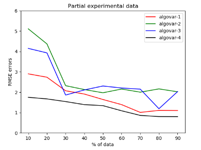
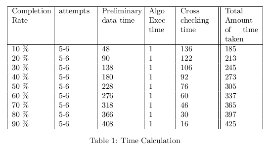
A set of experimental simulations where conducted on the data of patient 1, to have an understanding on the error given by the algorithm. In this simulations the amount of data given was varied, and the unknown data were predicted us- ing different algorithms. The simulations were conducted on 4 variations of the algorithm. 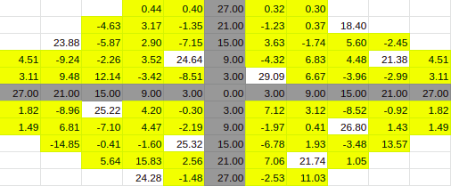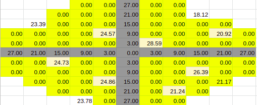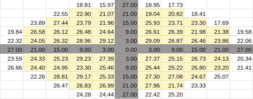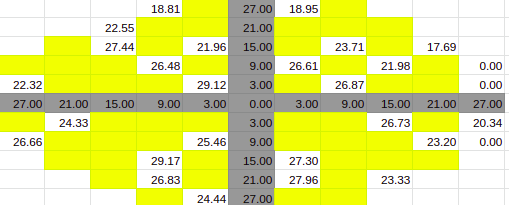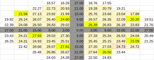The errors given by the 4 algorithms for this simulation along with the predicted time taken by the test for varying amount of data were noted and analyzed in table 1. It was conducted with 10% [8.1],20% [8.2],30% [8.3],40% [8.4],50% [8.5],60% [8.6],70% [8.7],80% [8.8] and 90% [8.9] of the data being filled.
 

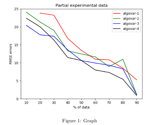
As you see in the graph [1] above, we get higher prediction rates or lower error rates as we have more data within a patient. We have not incorporated across the patient variation, just yet. The variation resulting from within patient analysis, is given as below in the simulations with varying levels of data from one patient. So at each level of data, we have corresponding partially filled data, predicted data and True(Actual) data. We have used 4 variations of the algorithms for each of the predicted values. We have compared the performance of these algorithms across various data levels in the graph [1] above.
 

10% Entries 

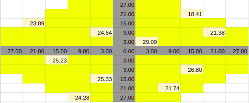
Estimate for 10% Entries from algoVar2 

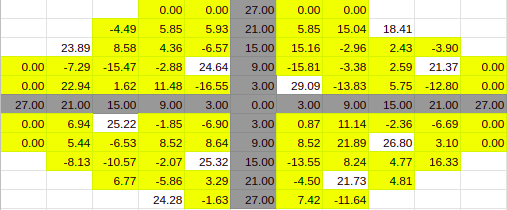
Estimate for 10% Entries from algoVar3 

Estimate for 10% Entries from algoVar4 

True Value for 10% 

30% Entries 

Estimate for 30% Entries from algoVar1 

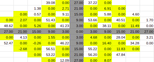
Estimate for 30% Entries from algoVar2 

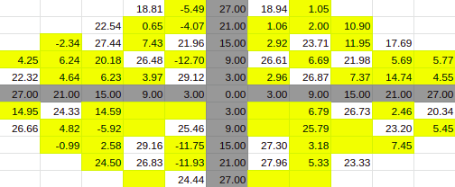
Estimate for 30% Entries from algoVar3 

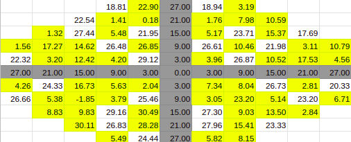
Estimate for 30% Entries from algoVar4 

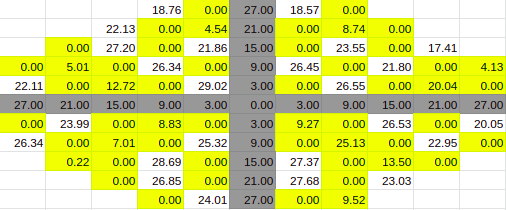
True Value for 30% 

60% Entries 

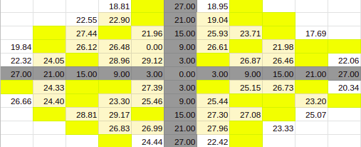
Estimate for 60% Entries from algoVar1 

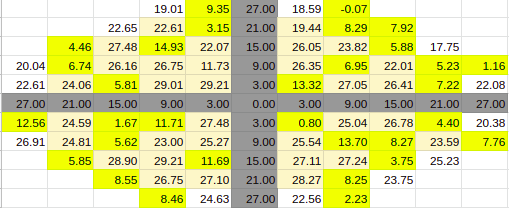
Estimate for 60% Entries from algoVar2 

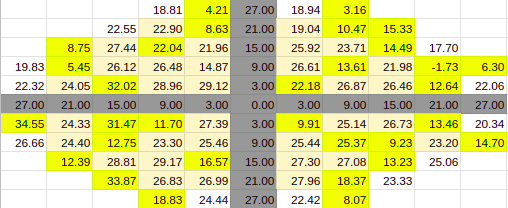
Estimate for 60% Entries from algoVar3 

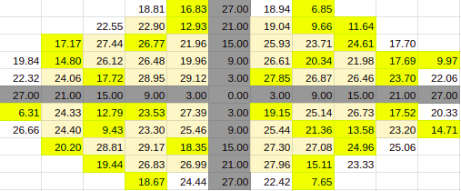
Estimate for 60% Entries from algoVar4 

True Value for 60% 

90% Entries 

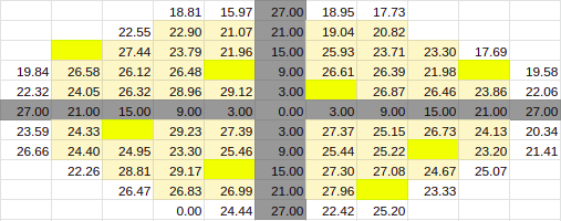
Estimate for 90% Entries from algoVar1 

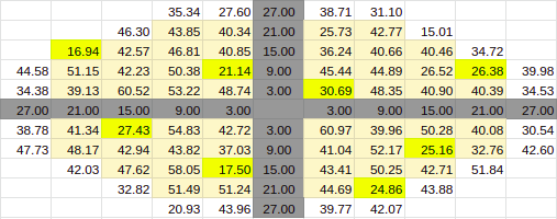
Estimate for 90% Entries from algoVar2 

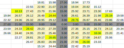
Estimate for 90% Entries from algoVar3 

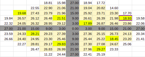
Estimate for 90% Entries from algoVar4 

True Value for 90% 

Across Patient Variation 

The simulation was conducted by taking the data of all the patients and stack- ing them all around the patient whose data was to be predicted. A 110 by 110 matrix was created and the data of all the patients were added into it as separate 11 by 11 matrices, thus allowing 100 patient data in the matrix. The patient’s data to be predicted was entered in the middle spot, thus it gets wrapped by all the known data.
If we look at each of the 11 by 11 matrix, they have some of the entries empty/zero due to the shape of the visual field. To prevent these points from having a negative effect we can change these values with the average value of their neighbouring two points. This should also be done for the blind spots and the axis points. This allows the matrix to have continuity.  

Further Implementation 

Our implementation is inspired by well-studied problems in the literature. Simply put; given an array or multiple arrays with some certain known entries, predict the remaining unknown entries such that your error is minimised. Our construct here is the collection of visual field intensity level thresholds, i.e. the minimum intensity level that a patient can see within their visual field, about their central line of focus. The center of this construct corresponds to what the fovea sees. The other peripheral edges of the construct correspond to the sensitivity of the other parts of the retina. If we do not impose certain conditions, this problem is underdetermined or impossible to solve. The condition we impose is that the known entries aren’t arbitrary. There is some level of dependency of the values we are trying to predict, on the already known entries.
This assumption is justified as intensity values around already known points would be highly correlated with each other. Mathematically speaking, we are trying to find a construct with values that exactly correspond to the ones we already have, in the same positions and whose rank is the minimum possible value achievable. This ensures that the predicted values which we get are as dependent on the values that we already have as possible.
This problem is said to be NP-hard which means that we cannot solve it in some reasonable time and checking whether or not the solution we proposed is correct would also not take a reasonable amount of time. Thus we can’t find the exact solution but employ an error-prone solution that can be definitely optimised, which gives us a chance at completing this construct, tolerably.  

Convex Relaxation 

We approach a solution to this problem by converting it to another, whose solution is not NP-hard. This is done by convex relaxation. Basically, the rank minimisation problem is non-convex, and is converted to a convex problem which we can solve in a reasonable time. Instead of minimising the rank of the matrix, we try and minimise the sum of the singular values of the matrix, It has been mathematically proven that if the number of entries that we know of is of the order of (around)
$$m \geq C \mu ^4nr^2(\log n)^2 \quad \quad \quad \quad \quad \quad (2)$$ or greater, where \(m < n\) is the number of entries of some square n × n matrix of rank r and some positive constant C, we can get a unique solution to minimising the nuclear norm of a matrix. This can be done by singular value thresholding. [12]  

Algorithms 

To tackle the problem of matrix completion, we will be exploring some well-established algorithms, discussed below.
 

Singular Value Thresholding 

This algorithm can be used in full effect whenever the nuclear norm minimum solution is the same as the lowest rank solution. The detailed algorithm steps can be understood in [12], but the bottom line is that from the already known matrix M with sparse points (implying low-rank), an estimate \(X^k\) can be constructed iteratively with k, filling up the unknown points. The singular values of \(X^k\) are obtained and at every iteration, by creating a proxy matrix \(Y^k\) whose singular values will be altered according to some tolerances and constraints to create \(X^k\). Once \(X^k\) is created, it should be the matrix with the smallest nuclear norm, approximating a low rank M .
 

Latent Factor Based Method 

This approach looks at the sparse matrix M in a different light. This method was made popular by the Netflix problem winners. The matrix M can be thought of as consisting of row-wise of users, rating column wise items, as shown below.
 

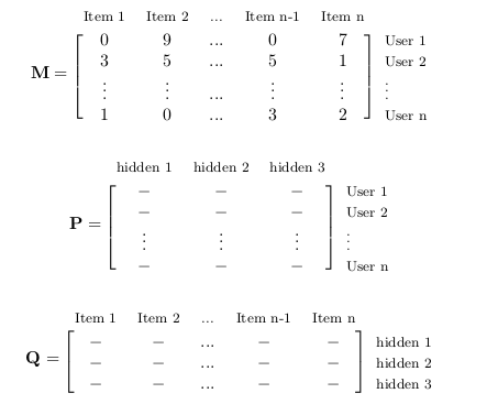
$$ M=PQ \quad \quad \quad \quad \quad \quad \quad \quad \quad (3)$$ This n × n matrix, M can be f actored as the product of two other matrices P and Q, which are n × r and r × n in size, respectively. Here, r represents some hidden or latent factors, which contribute to the construction of M . If M represents user ratings or eye sensitivity levels, they are mathematically the same sparse matrix.
We can see from the matrices above that every rating is nothing the combination of the rows of P and the columns of Q. Thus, we can get an approximation of M by constructing \(\hat{P}\) and \(\hat{Q}\) such that \(\hat{P}\) \(\hat{Q}\) = \(\hat{M} \simeq M .\) If every known entry of M is denoted by m, it would mathematically imply solving the following problem. $$\min_{\forall q,p} \sum_{(\forall m_{kl} \neq 0) \in M}{}{(m_{kl}-p_{kl}q_{kl})}^2 \quad \quad \quad \quad \quad \quad (4)$$  

Alternating Least Squares 

Equation 4 is a quadratic convex optimisation problem, which can be solved by fixing p and finding q, then fixing q and fining p, and so on. This method of alternating between p and q is well documented and used to find the values of P and Q to reconstruct the matrix M . It’s called the alternating least squares method as you alternate between two unknowns while solving a least squares problem.
 

Biased Alternating Least Squares 

While trying to solve the alternating least squares problems, the many constraints involved lead to multiple solutions that don’t often capture reality. This is due to an artificial bias added while running the alternating least squares algorithm.
To combat this, the Biased Alternating Least Squares, intelligently removes the bias, thereby helping accuracies improve.  

References 

[1] Visual Field Digest, Haag Streit Handbook, 2016 Ref
[2] Andrew Turpin, Allison M. McKendrick, Chris A. Johnson, and Algis J. Vingrys. Properties of Perimetric Threshold Estimates from Full Threshold, ZEST, and SITA-like Strategies, as Determined by Computer Simulation. Investigative Ophthalmology and Visual Science, November 2003 Ref
[3] Andrew J. Anderson. Spatial Resolution of the Tendency-Oriented Perimetry Algorithm. From Discoveries in Sight, Devers Eye Institute, Portland Oregon, (2002) Ref
[4] https://webeye.ophth.uiowa.edu/ips/Perimetr.htm
[5] https://www.perimetry.org/index.php/perimetry
[6] Boel Bengtsson, Anders Heijl and Jonny Olsson. Evaluation of a new threshold visual field strategy, SITA, in normal subjects. Acta Ophthalmol. Scand. 1998 Ref
[7] ALGIS J,VINGRYS,Phd,FAAO,MICHEAL J.PLANTA, MOptom. A New Look at Threshold Estimation Algorithms for Automated Static Perimetry.1999 Ref
[8] Andrew Turpin, Allison M. McKendrick, Chris A. Johnson, and Algis J. Vingrys. Properties of Perimetric Threshold Estimates from Full Threshold, ZEST, and SITA-like Strategies, as Determined by Computer Simulation. Nov 2003 Ref
[9] Boel Bengtsson, Anders Heijl and Jonny Olsson. Evaluation of a new threshold visual field strategy, SITA, in normal subjects. Acta Ophthalmol. Scand. 1998 Ref
[10] Andrew J.Anderson. Spatial Resolution of the Tendency-Oriented Perimetry Algorithm. May 2003. Ref [11] Nikki J. Rubinstein, Allison M. McKendrick, and Andrew Turpin. Incorporating Spatial Models in Visual Field Test Procedures. Mar 2016 Ref
[12] A Singular Value Thresholding Algorithm for Matrix Completion Jian Feng Cai, Emmanuel J. Candes, Zuowei Shen Ref